Generative Adversarial Networks Part 2 — Improved Image Generation using Deep Convolutional GAN (DC GAN)
In Part 1 of our Generational Adversarial Networks Series, we saw what GANs typically are and how to implement the simple GAN using Python and Pytorch.
In this part, we will implement a bigger type of GAN called the Deep Convolutional GAN, or DCGAN for short. DC Gan uses Convolutional Layers to generate better images than our linear layered model since Convolutional layers are better at generalizing image data. So, let’s get right into this.
What are Convolutional Layers
By Deep Convolutional NN we mean that the Neural Network consists of many Convolutional Layers. But what exactly are convolutional layers? To understand this, let’s take the image of a car.

Now this image has many different features using which we can assume that this is the image of a car. For example tires, edges of the car, window screen, Front bumper, etc. But Linear Layers cannot see these features because we pass in the pixel value of each pixel as an input feature. Only the pixel value cannot determine these features. Althought his approach works for smaller images like the mnist one we saw in the first part, yet for bigger images or high resolution images, this approach will fail. You can even confirm this by trying to train the simple-gan from the first part on the cifar10 dataset which contains images in 3 color channels.
So what’s the solution then? Convolutional Neural Networks. The Convolutional Neural Networks work by splitting the image into smaller and smaller sub images or features using a filter (also called a kernel). Then these features are individually identified as the tires, or window screens of a car or a handle of a mug or any other feature which can then be classified or generalized with increased accuracy.
You can see these features and kernels in action on the CNN Explainer.

Here you can see the individual sub images or features being extracted for every single channel in the image. Let’s take a deeper look at all the parameters. There are usually 5 parameters given to a convolutional layer:
- in_channels
- out_channels
- kernel_size
- stride
- padding
in_channels
This corresponds to the number of channels the input image or the input feature has for example in our car case we have 3 input channels i.e. RGB channels. These channels will be increased as we move deep in the convolutional neural network.
out_channels
The number of output channels for the layer, for example in the figure above we have 10 output channels for our car image so 10 sub-images or features from the input channels are being obtained.
kernel_size
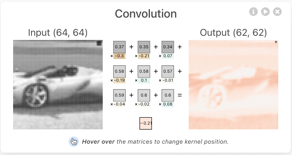
The size of the kernel which extracts the features. Typically this value is 3 or 4 but can vary depending on the model architecture. The kernel corresponds to the filer that is applied to the input channel to find the corresponding output channel.

the 3×3 kernel or simply put a 3×3 vector goes through every pixel of the image and performs calculation (Usually adding the kernel value and the pixel value) and returns the result. This result then adds up from all the input channels to form a single subimage or feature.
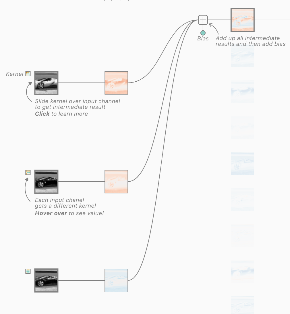
Each kernel is trained to find a different feature for example extracting the edges, extracting the tire edges, extracting the face or nose etc. A kernel typically looks like [[0.2, 0.1, 0.423], [0.5, 0.3, 0.7], [0.12, 0.354, 0.243]].
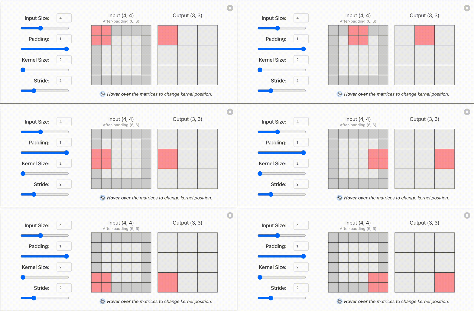
stride and padding
The stride and padding are two other parameters that influence the output of the Convolution Layer. The stride corresponds to the shift in the window from the previous location. For example, suppose a kernel of size 3 is sitting on the image on pixel no (0, 0) to (2, 2) meaning 9 pixels, then a stride of 2 means the next iteration will be from (0, 2) to (2, 4) meaning again 9 pixels but the pixels (0,2),(1,2),(2,2) are repeated. The padding parameter adds extra pixels around the image, for example a padding of 1 adds 1 extra pixel around the whole image on all the sides. You can take a deeper look at padding and stride from this gif taken from the CNN Explainer website. You can also play around with these parameters from the CNN Expaliner website.
These layers go on and on until enough features are extracted. Then in a conventional CNN like the tinyVGG Model, at the end a Fully connected Neural Network with Linear Layers is attached for classification purposes. But for this tutorial we will not use a Fully connected NN at the end. Rather we will create the generator and discriminator purely from Convolutional Layers.
Since now we have a pretty good idea of what Convolutions are, Let’s get into building our DC GAN.
Building DC-GAN
The code that we are going to write in this article is also available on my GitHub repository https://github.com/Zohaibb-m/the-ultimate-GAN/tree/main/the_ultimate_gan/models/dc_gan . If during this blog, something doesn’t work. You can open an issue on my GitHub repository and we can discuss the issue there.
The architecture of DC GAN’s generator model as shown in the research paper is
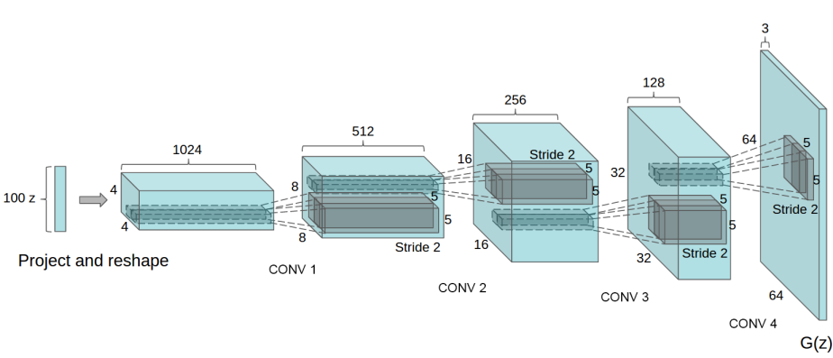
For the discriminator, We just have to reverse this architecture and use Transposed Convolutional Layers to get from an image to a single neuron outputting the fakeness of the generated image.
Building the Discriminator
Let’s start coding. First, we will import the required libraries:
import torch
from torch import nn
from torchinfo import summary
We will use the torch for tensor operations and torch.nn to lay down our foundation for the NN. The purpose of torchinfo will be explained later.
Now for the discriminator code:
class Discriminator(nn.Module):
    def __init__(self, in_channels, mid_channels, out_channels):
        super().__init__()
        self.model = nn.Sequential(
            *self.discriminator_block(in_channels, mid_channels, normalize=False),
            *self.discriminator_block(mid_channels, mid_channels * 2),
            *self.discriminator_block(mid_channels * 2, mid_channels * 4),
            *self.discriminator_block(mid_channels * 4, mid_channels * 8),
            nn.Conv2d(mid_channels * 8, out_channels, 4, 2, 0),
            nn.Sigmoid()
        )

    @staticmethod
    def discriminator_block(in_channels, out_channels, normalize=True):
        return nn.Sequential(
            nn.Conv2d(
                in_channels=in_channels,
                out_channels=out_channels,
                kernel_size=4,
                stride=2,
                padding=1,
            ),
            nn.BatchNorm2d(out_channels) if normalize else nn.Identity(),
            nn.LeakyReLU(0.2),
        )

    def forward(self, x):
        return self.model(x)
First, let’s take a look at the discriminator block
def discriminator_block(in_channels, out_channels, normalize=True):
    return nn.Sequential(
        nn.Conv2d(
            in_channels=in_channels,
            out_channels=out_channels,
            kernel_size=4,
            stride=2,
            padding=1,
        ),
        nn.BatchNorm2d(out_channels) if normalize else nn.Identity(),
        nn.LeakyReLU(0.2),
    )
The discriminator block is the fundamental building block of the Discriminator and contains 3 layers. The Conv2d layer does what was explained earlier. Taken in the image, extract features from the input_channels and return the output. Then there is the BatchNorm Layer. The batchnorm layer is already explained In the first part so we will keep it brief here. It is used to help normalize the neurons and fix the internal covariate shift problem. Then comes the last layer, the LeakyReLU which is responsible for adding nonlinearity so the model can better generalize the pattern of data. One thing to mention is we are also getting a normalize parameter. This parameter is used when we don’t want to add the BatchNorm layer since in the first block we don’t usually need it because the data is already coming normalized.
Pretty straightforward. Now let’s look at the overall discriminator.
self.model = nn.Sequential(
    *self.discriminator_block(in_channels, mid_channels, normalize=False),
    *self.discriminator_block(mid_channels, mid_channels * 2),
    *self.discriminator_block(mid_channels * 2, mid_channels * 4),
    *self.discriminator_block(mid_channels * 4, mid_channels * 8),
    nn.Conv2d(mid_channels * 8, out_channels, 4, 2, 0),
    nn.Sigmoid()
)
We have the first layer normalized = false so that it doesn’t contain the batch norm layer since the data is already normalized. Then we have 3 more discriminator blocks. At each block, we are increasing the output_channels so that more and more features are extracted. Finally, in the end, we have the last Convolutional Layer which returns only 1 output_channel. The size of this will be (1, 1, 1, 1) Meaning the fakeness of the image. The sigmoid at the end scales it between 0 and 1. Keep in mind that at each layer the size of the feature image gets smaller and smaller until the end where the final size of the output is 1 float depicting the fakeness of the image.
Finally, we have the forward function.
def forward(self, x):
    return self.model(x)
Building the Generator
Now let’s build the generator. The full code for the generator is:
class Generator(nn.Module):
    def __init__(self, latent_dim: int, mid_channels: int, out_channels: int):
        super().__init__()
        self.model = nn.Sequential(
            *self.generator_block(
                latent_dim,
                mid_channels * 16,
                kernel=4,
                stride=2,
                padding=1,
                normalize=False,
            ),
            *self.generator_block(mid_channels * 16, mid_channels * 8),
            *self.generator_block(mid_channels * 8, mid_channels * 4),
            *self.generator_block(mid_channels * 4, mid_channels * 2),
            *self.generator_block(mid_channels * 2, mid_channels),
            nn.ConvTranspose2d(
                mid_channels, out_channels, kernel_size=4, stride=2, padding=1
            ),
            nn.Tanh()
        )

    @staticmethod
    def generator_block(in_channels, out_channels, kernel=4, stride=2, padding=1, normalize=True):
        return nn.Sequential(
            nn.ConvTranspose2d(in_channels, out_channels, kernel, stride, padding,),
            nn.BatchNorm2d(num_features=out_channels) if normalize else nn.Identity(),
            nn.ReLU(inplace=True),
        )

    def forward(self, x):
        return self.model(x)
That’s a little too much to digest right away, but let’s see each line and its purpose. First, let’s look at the generator block:
def generator_block(in_channels, out_channels, kernel=4, stride=2, padding=1, normalize=True):
        return nn.Sequential(
            nn.ConvTranspose2d(in_channels, out_channels, kernel, stride, padding,),
            nn.BatchNorm2d(num_features=out_channels) if normalize else nn.Identity(),
            nn.ReLU(inplace=True),
        )
The generator block is the building block for our generator and contains 3 layers. The ConvTranspose2d layer, The batch norm layer, and the ReLU activation layer. The batchnorm and ReLU are straightforward so I will only explain the ConvTranspose2d layer in detail.
The ConvTranspose2d Layer
This layer is used for upscaling contrary to what Convolution Layer does. Although this is not the exact opposite, this also uses kernel_size, stride, and padding parameters to upscale the image to a higher dimension. It takes pixel values under the kernel and multiplies them with the kernel, adds all the RGB channels, and produces a final upscaled output. This can be visualized from the following GitHub repository.
Now, let’s look at the overall generator:
self.model = nn.Sequential(
    *self.generator_block(
        latent_dim,
        mid_channels * 16,
        kernel=4,
        stride=2,
        padding=1,
        normalize=False,
    ),
    *self.generator_block(mid_channels * 16, mid_channels * 8),
    *self.generator_block(mid_channels * 8, mid_channels * 4),
    *self.generator_block(mid_channels * 4, mid_channels * 2),
    *self.generator_block(mid_channels * 2, mid_channels),
    nn.ConvTranspose2d(
        mid_channels, out_channels, kernel_size=4, stride=2, padding=1
    ),
    nn.Tanh()
)
We first have a generator block with normalize=false again due to the reason that the input data is already normalized. Then we have 4 generator blocks each upscaling the output channels but double the previous channels. Finally, we have the last layer which again with different padding and stride gives us a final output of (batch size, 3, 64, 64). This is the output shape. Lastly, Tanh scales the output between -1 and 1. This is because we apply a normalization of 0.5 and 0.5 on each image which also outputs values between -1 and 1.
Putting everything together
Let’s move to the final piece of our model, putting everything together in a class. The complete code for this part is here:
import torch
import torchvision
import os

from torch import nn
from torch import optim
from torchvision import datasets, transforms
from torch.utils.data import DataLoader
from torch.utils.tensorboard import SummaryWriter
from torchinfo import summary
from the_ultimate_gan.models.dc_gan.layers import Discriminator, Generator
from tqdm import tqdm

class DCGAN:
    def __init__(self, learning_rate: float, latent_dim: int, batch_size: int, num_epochs: int):
        self.current_epoch = None
        self.writer_real = None
        self.writer_fake = None
        self.criterion = None
        self.opt_gen = None
        self.opt_disc = None
        self.discriminator = None
        self.generator = None
        self.latent_dim = latent_dim
        self.batch_size = batch_size
        self.num_epochs = num_epochs

        self.device = torch.device(
            "cuda"
            if torch.cuda.is_available()
            else "mps" if torch.backends.mps.is_available() else "cpu"
        )
        self.out_channels = 1

        # Define the transforms
        self.transform = transforms.Compose(
            [
                transforms.Resize(64),
                transforms.CenterCrop(64),
                transforms.ToTensor(),
                (
                    transforms.Normalize(
                        [0.5 for _ in range(self.out_channels)],
                        [0.5 for _ in range(self.out_channels)],
                    )
                ),
            ]
        )

        # Set the seed for reproducibility
        torch.manual_seed(42)
        # Generate fixed noise for generating images later
        self.fixed_noise = torch.randn((self.batch_size, self.latent_dim, 1, 1)).to(
            self.device
        )

        self.dataset = datasets.MNIST(
            root="Data/", transform=self.transform, download=True
        )

        # Create a data loader
        self.loader = DataLoader(self.dataset, batch_size=self.batch_size, shuffle=True)

        self.init_generator(latent_dim, self.out_channels)  # Initialize the generator

        self.init_discriminator(self.out_channels)  # Initialize the discriminator

        self.init_optimizers(learning_rate)  # Initialize the optimizers

        self.init_loss_fn()  # Initialize the loss function

        self.init_summary_writers()  # Initialize the tensorboard writers

        # Print the model configurations
        print(
            f"Model DC GAN Loaded with dataset: {dataset}. The following configurations were used:\nLearning Rate: {learning_rate}, Epochs: {num_epochs}, Batch Size: {batch_size}, Transforms with Mean: 0.5 and Std: 0.5 for each Channel.\n Starting the Model Training now."
        )

    def init_generator(self, latent_dim, out_channels):
        self.generator = Generator(latent_dim, 64, out_channels).to(
            self.device
        )  # Initialize the generator
        self.generator.apply(weights_init)

    def init_discriminator(self, in_channels):
        self.discriminator = Discriminator(in_channels, 64, 1).to(
            self.device
        )  # Initialize the discriminator
        self.discriminator.apply(weights_init)

    def init_optimizers(self, learning_rate):
        self.opt_disc = optim.Adam(
            self.discriminator.parameters(), lr=learning_rate, betas=(0.5, 0.999)
        )  # Initialize the discriminator optimizer
        self.opt_gen = optim.Adam(
            self.generator.parameters(), lr=learning_rate, betas=(0.5, 0.999)
        )  # Initialize the generator optimizer

    def init_loss_fn(self):
        self.criterion = nn.BCELoss()  # Initialize the loss function

    def init_summary_writers(self):
        self.writer_fake = SummaryWriter(
            f"runs/GAN_{self.dataset_name}/fake"
        )  # Initialize the tensorboard writer for fake images
        self.writer_real = SummaryWriter(
            f"runs/GAN_{self.dataset_name}/real"
        )  # Initialize the tensorboard writer for real images

    def train(self):
        try:
            step = 0  # Step for the tensorboard writer
            self.current_epoch = 1  # Initialize the current epoch
            while (
                self.current_epoch <= self.num_epochs
            ):  # Loop over the dataset multiple times
                for batch_idx, (real, _) in enumerate(
                    tqdm(self.loader)
                ):  # Get the inputs; data is a list of [inputs, labels]
                    real = real.to(self.device)  # Move the data to the device
                    batch_size = real.shape[0]  # Get the batch size

                    noise = torch.randn((batch_size, self.latent_dim, 1, 1)).to(
                        self.device
                    )  # Generate random noise
                    fake = self.generator(noise)  # Generate fake images

                    discriminator_real = self.discriminator(real)
                    loss_d_real = self.criterion(
                        discriminator_real, torch.ones_like(discriminator_real)
                    )  # Calculate the loss for real images

                    discriminator_fake = self.discriminator(fake).view(
                        -1
                    )  # Get the discriminator output for fake images
                    loss_d_fake = self.criterion(
                        discriminator_fake, torch.zeros_like(discriminator_fake)
                    )  # Calculate the loss for fake images
                    loss_discriminator = (
                        loss_d_real + loss_d_fake
                    ) / 2  # Calculate the average loss for the discriminator

                    self.discriminator.zero_grad()  # Zero the gradients
                    loss_discriminator.backward(
                        retain_graph=True
                    )  # Backward pass for the discriminator
                    self.opt_disc.step()  # Update the discriminator weights

                    output = self.discriminator(fake).view(
                        -1
                    )  # Get the discriminator output for fake images
                    loss_generator = self.criterion(
                        output, torch.ones_like(output)
                    )  # Calculate the loss for the generator
                    self.generator.zero_grad()  # Zero the gradients
                    loss_generator.backward()  # Backward pass for the generator
                    self.opt_gen.step()  # Update the generator weights

                    if batch_idx == 0:
                        print(
                            f"Epoch [{self.current_epoch}/{self.num_epochs}] Loss Discriminator: {loss_discriminator:.8f}, Loss Generator: {loss_generator:.8f}"
                        )

                        with torch.no_grad():  # Save the generated images to tensorboard
                            fake = self.generator(
                                self.fixed_noise
                            )  # Generate fake images
                            data = real  # Get the real images
                            img_grid_fake = torchvision.utils.make_grid(
                                fake, normalize=True
                            )  # Create a grid of fake images
                            img_grid_real = torchvision.utils.make_grid(
                                data, normalize=True
                            )  # Create a grid of real images

                            self.writer_fake.add_image(
                                f"{self.dataset_name} Fake Images",
                                img_grid_fake,
                                global_step=step,
                            )  # Add the fake images to tensorboard
                            self.writer_real.add_image(
                                f"{self.dataset_name} Real Images",
                                img_grid_real,
                                global_step=step,
                            )  # Add the real images to tensorboard
                            step += 1  # Increment the step


    @staticmethod
    def get_model_summary(summary_model, input_shape) -> summary:
        return summary(
            summary_model,
            input_size=input_shape,
            verbose=0,
            col_names=["input_size", "output_size", "num_params", "trainable"],
            col_width=20,
            row_settings=["var_names"],
        )


def weights_init(m):
    class_name = m.__class__.__name__
    if class_name.find("Conv") != -1:
        nn.init.normal_(m.weight.data, 0.0, 0.02)
    elif class_name.find("BatchNorm") != -1:
        nn.init.normal_(m.weight.data, 1.0, 0.02)
        nn.init.constant_(m.bias.data, 0)


if __name__ == "__main__":
    model = DCGAN(2e-4, 100, 128, 50)
    model.train()
Most of the code is pretty straightforward and is already explained in part 1 of this series. We’ll do a brief look over the code now:
self.current_epoch = None
self.writer_real = None
self.writer_fake = None
self.criterion = None
self.opt_gen = None
self.opt_disc = None
self.discriminator = None
self.generator = None
self.latent_dim = latent_dim
self.batch_size = batch_size
self.num_epochs = num_epochs

self.device = torch.device(
    "cuda"
    if torch.cuda.is_available()
    else "mps" if torch.backends.mps.is_available() else "cpu"
)
self.out_channels = 1
Initializing the required class variables and setting device agnostic code so that GPU is used whenever available.
# Define the transforms
self.transform = transforms.Compose(
    [
        transforms.Resize(64),
        transforms.CenterCrop(64),
        transforms.ToTensor(),
        (
            transforms.Normalize(
                [0.5 for _ in range(self.out_channels)],
                [0.5 for _ in range(self.out_channels)],
            )
        ),
    ]
)
Defining the transformation that will be applied to the whole dataset. Here the notable points are the 2 for loops. This is necessary since until now we were working with images with 1 channel but now we will also be working with images with RGB color channels so in that case we define the mean and std for each channel. So if we want to train some other dataset like the CELEBA dataset, we will set the self.out_channels to 3.
# Set the seed for reproducibility
torch.manual_seed(42)
# Generate fixed noise for generating images later
self.fixed_noise = torch.randn((self.batch_size, self.latent_dim, 1, 1)).to(
    self.device
)

self.dataset = datasets.MNIST(
    root="Data/", transform=self.transform, download=True
)

# Create a data loader
self.loader = DataLoader(self.dataset, batch_size=self.batch_size, shuffle=True)
We set the manual seed for the reproducibility of results and create a fixed noise that will be used to evaluate our generator’s training. Then we initialize the dataset using torchvision.datasets sub-module and then create a dataloader from this dataset.
self.init_generator(latent_dim, self.out_channels)  # Initialize the generator

self.init_discriminator(self.out_channels)  # Initialize the discriminator

self.init_optimizers(learning_rate)  # Initialize the optimizers

self.init_loss_fn()  # Initialize the loss function

self.init_summary_writers()  # Initialize the tensorboard writers

# Print the model configurations
print(
    f"Model DC GAN Loaded with dataset Mnist. The following configurations were used:\nLearning Rate: {learning_rate}, Epochs: {num_epochs}, Batch Size: {batch_size}, Transforms with Mean: 0.5 and Std: 0.5 for each Channel.\n Starting the Model Training now."
)
Initializing the generators, discriminators, optimizers, and the loss fn. The loss function logic is the same as Part 1 so we will not discuss it here today. Finally, we initialize the summary writer and that is it for our model’s constructor.
def train(self):
  try:
      step = 0  # Step for the tensorboard writer
      self.current_epoch = 1  # Initialize the current epoch
      while (
          self.current_epoch <= self.num_epochs
      ):  # Loop over the dataset multiple times
          for batch_idx, (real, _) in enumerate(
              tqdm(self.loader)
          ):  # Get the inputs; data is a list of [inputs, labels]
              real = real.to(self.device)  # Move the data to the device
              batch_size = real.shape[0]  # Get the batch size

              noise = torch.randn((batch_size, self.latent_dim, 1, 1)).to(
                  self.device
              )  # Generate random noise
              fake = self.generator(noise)  # Generate fake images

              discriminator_real = self.discriminator(real)
              loss_d_real = self.criterion(
                  discriminator_real, torch.ones_like(discriminator_real)
              )  # Calculate the loss for real images

              discriminator_fake = self.discriminator(fake).view(
                  -1
              )  # Get the discriminator output for fake images
              loss_d_fake = self.criterion(
                  discriminator_fake, torch.zeros_like(discriminator_fake)
              )  # Calculate the loss for fake images
              loss_discriminator = (
                  loss_d_real + loss_d_fake
              ) / 2  # Calculate the average loss for the discriminator

              self.discriminator.zero_grad()  # Zero the gradients
              loss_discriminator.backward(
                  retain_graph=True
              )  # Backward pass for the discriminator
              self.opt_disc.step()  # Update the discriminator weights

              output = self.discriminator(fake).view(
                  -1
              )  # Get the discriminator output for fake images
              loss_generator = self.criterion(
                  output, torch.ones_like(output)
              )  # Calculate the loss for the generator
              self.generator.zero_grad()  # Zero the gradients
              loss_generator.backward()  # Backward pass for the generator
              self.opt_gen.step()  # Update the generator weights

              if batch_idx == 0:
                  print(
                      f"Epoch [{self.current_epoch}/{self.num_epochs}] Loss Discriminator: {loss_discriminator:.8f}, Loss Generator: {loss_generator:.8f}"
                  )

                  with torch.no_grad():  # Save the generated images to tensorboard
                      fake = self.generator(
                          self.fixed_noise
                      )  # Generate fake images
                      data = real  # Get the real images
                      img_grid_fake = torchvision.utils.make_grid(
                          fake, normalize=True
                      )  # Create a grid of fake images
                      img_grid_real = torchvision.utils.make_grid(
                          data, normalize=True
                      )  # Create a grid of real images

                      self.writer_fake.add_image(
                          f"{self.dataset_name} Fake Images",
                          img_grid_fake,
                          global_step=step,
                      )  # Add the fake images to tensorboard
                      self.writer_real.add_image(
                          f"{self.dataset_name} Real Images",
                          img_grid_real,
                          global_step=step,
                      )  # Add the real images to tensorboard
                      step += 1  # Increment the step
This is the train function and is the same as the simple gan. We take the real image, create a noise, and pass it to the generator to create a fake image, then we pass both to BCE loss one by one calculate discriminator loss, and update the discriminator weights. Similarly, we take the noise, generate it through the generator, and ask the discriminator to identify it. Based on that, we calculate the generator loss and update its parameters. Finally, there are some epoch and loss updates printing stuff and summary writing code for tensorboard. This is it for the train function.
def get_model_summary(summary_model, input_shape) -> summary:
        return summary(
            summary_model,
            input_size=input_shape,
            verbose=0,
            col_names=["input_size", "output_size", "num_params", "trainable"],
            col_width=20,
            row_settings=["var_names"],
        )

def weights_init(m):
    class_name = m.__class__.__name__
    if class_name.find("Conv") != -1:
        nn.init.normal_(m.weight.data, 0.0, 0.02)
    elif class_name.find("BatchNorm") != -1:
        nn.init.normal_(m.weight.data, 1.0, 0.02)
        nn.init.constant_(m.bias.data, 0)
These are the two extra functions. The weights_init function is used to initialize the weights according to the original author of the DCGAN research paper. The get_model_summary is a very interesting function. It uses the torchinfo library we imported earlier to get the summary of the model. We will directly use it in action to see its power. This is for the coding part, let’s now see our model in action. First, create the model object, and then let’s call the get_model_summary function to get the generator model details.
model = DCGAN(2e-4, 100, 128, 50, "cifar10", 100, False)
print(model.get_model_summary(model.generator, (1, 100, 1, 1)))
========================================================================================================================
Layer (type (var_name)) Input Shape Output Shape Param # Trainable
========================================================================================================================
Generator (Generator) [1, 100, 1, 1] [1, 3, 64, 64] -- True
├─Sequential (model) [1, 100, 1, 1] [1, 3, 64, 64] -- True
│ └─ConvTranspose2d (0) [1, 100, 1, 1] [1, 1024, 2, 2] 1,639,424 True
│ └─Identity (1) [1, 1024, 2, 2] [1, 1024, 2, 2] -- --
│ └─ReLU (2) [1, 1024, 2, 2] [1, 1024, 2, 2] -- --
│ └─ConvTranspose2d (3) [1, 1024, 2, 2] [1, 512, 4, 4] 8,389,120 True
│ └─BatchNorm2d (4) [1, 512, 4, 4] [1, 512, 4, 4] 1,024 True
│ └─ReLU (5) [1, 512, 4, 4] [1, 512, 4, 4] -- --
│ └─ConvTranspose2d (6) [1, 512, 4, 4] [1, 256, 8, 8] 2,097,408 True
│ └─BatchNorm2d (7) [1, 256, 8, 8] [1, 256, 8, 8] 512 True
│ └─ReLU (8) [1, 256, 8, 8] [1, 256, 8, 8] -- --
│ └─ConvTranspose2d (9) [1, 256, 8, 8] [1, 128, 16, 16] 524,416 True
│ └─BatchNorm2d (10) [1, 128, 16, 16] [1, 128, 16, 16] 256 True
│ └─ReLU (11) [1, 128, 16, 16] [1, 128, 16, 16] -- --
│ └─ConvTranspose2d (12) [1, 128, 16, 16] [1, 64, 32, 32] 131,136 True
│ └─BatchNorm2d (13) [1, 64, 32, 32] [1, 64, 32, 32] 128 True
│ └─ReLU (14) [1, 64, 32, 32] [1, 64, 32, 32] -- --
│ └─ConvTranspose2d (15) [1, 64, 32, 32] [1, 3, 64, 64] 3,075 True
│ └─Tanh (16) [1, 3, 64, 64] [1, 3, 64, 64] -- --
========================================================================================================================
Total params: 12,786,499
Trainable params: 12,786,499
Non-trainable params: 0
Total mult-adds (M): 556.15
========================================================================================================================
Input size (MB): 0.00
Forward/backward pass size (MB): 2.10
Params size (MB): 51.15
Estimated Total Size (MB): 53.24
========================================================================================================================Woohoo! We built a multi-million parameter model. The total parameters of our generator model are 12.78 Million. Pretty cool right? You can also see the different output shapes of different layers. Now let’s also see our discriminator model’s details.
========================================================================================================================
Layer (type (var_name))                  Input Shape          Output Shape         Param #              Trainable
========================================================================================================================
Discriminator (Discriminator)            [1, 3, 64, 64]       [1, 1, 1, 1]         --                   True
├─Sequential (model)                     [1, 3, 64, 64]       [1, 1, 1, 1]         --                   True
│    └─Conv2d (0)                        [1, 3, 64, 64]       [1, 64, 32, 32]      3,136                True
│    └─Identity (1)                      [1, 64, 32, 32]      [1, 64, 32, 32]      --                   --
│    └─LeakyReLU (2)                     [1, 64, 32, 32]      [1, 64, 32, 32]      --                   --
│    └─Conv2d (3)                        [1, 64, 32, 32]      [1, 128, 16, 16]     131,200              True
│    └─BatchNorm2d (4)                   [1, 128, 16, 16]     [1, 128, 16, 16]     256                  True
│    └─LeakyReLU (5)                     [1, 128, 16, 16]     [1, 128, 16, 16]     --                   --
│    └─Conv2d (6)                        [1, 128, 16, 16]     [1, 256, 8, 8]       524,544              True
│    └─BatchNorm2d (7)                   [1, 256, 8, 8]       [1, 256, 8, 8]       512                  True
│    └─LeakyReLU (8)                     [1, 256, 8, 8]       [1, 256, 8, 8]       --                   --
│    └─Conv2d (9)                        [1, 256, 8, 8]       [1, 512, 4, 4]       2,097,664            True
│    └─BatchNorm2d (10)                  [1, 512, 4, 4]       [1, 512, 4, 4]       1,024                True
│    └─LeakyReLU (11)                    [1, 512, 4, 4]       [1, 512, 4, 4]       --                   --
│    └─Conv2d (12)                       [1, 512, 4, 4]       [1, 1, 1, 1]         8,193                True
│    └─Sigmoid (13)                      [1, 1, 1, 1]         [1, 1, 1, 1]         --                   --
========================================================================================================================
Total params: 2,766,529
Trainable params: 2,766,529
Non-trainable params: 0
Total mult-adds (M): 103.94
========================================================================================================================
Input size (MB): 0.05
Forward/backward pass size (MB): 1.44
Params size (MB): 11.07
Estimated Total Size (MB): 12.56
========================================================================================================================
Our discriminator is much smaller than the generator with only 2.7 Million parameters. Now let’s call the train function to train our model.
model.train()And this is the output of the first few epochs:
  0%|          | 0/391 [00:00<?, ?it/s]
Epoch [1/50] Loss Discriminator: 0.92446613, Loss Generator: 9.94396973
100%|██████████| 391/391 [00:41<00:00,  9.34it/s]
  0%|          | 0/391 [00:00<?, ?it/s]
Epoch [2/50] Loss Discriminator: 0.57567698, Loss Generator: 11.49219131
100%|██████████| 391/391 [00:41<00:00,  9.35it/s]
  0%|          | 0/391 [00:00<?, ?it/s]
Epoch [3/50] Loss Discriminator: 0.27977556, Loss Generator: 3.70662141
100%|██████████| 391/391 [00:41<00:00,  9.35it/s]
  0%|          | 0/391 [00:00<?, ?it/s]
Epoch [4/50] Loss Discriminator: 0.30883747, Loss Generator: 5.79522896
100%|██████████| 391/391 [00:41<00:00,  9.36it/s]
  0%|          | 0/391 [00:00<?, ?it/s]
Epoch [5/50] Loss Discriminator: 0.57482171, Loss Generator: 2.80262351
100%|██████████| 391/391 [00:41<00:00,  9.36it/s]
  0%|          | 0/391 [00:00<?, ?it/s]
Epoch [6/50] Loss Discriminator: 0.30429140, Loss Generator: 2.44376278
100%|██████████| 391/391 [00:41<00:00,  9.37it/s]
  0%|          | 0/391 [00:00<?, ?it/s]
Epoch [7/50] Loss Discriminator: 0.44996336, Loss Generator: 1.89657700
100%|██████████| 391/391 [00:41<00:00,  9.38it/s]
  0%|          | 0/391 [00:00<?, ?it/s]
Epoch [8/50] Loss Discriminator: 0.80704874, Loss Generator: 0.99019194
100%|██████████| 391/391 [00:41<00:00,  9.38it/s]
  0%|          | 0/391 [00:00<?, ?it/s]
Epoch [9/50] Loss Discriminator: 1.25493765, Loss Generator: 5.55383682
100%|██████████| 391/391 [00:41<00:00,  9.37it/s]
  0%|          | 0/391 [00:00<?, ?it/s]
Epoch [10/50] Loss Discriminator: 0.28618163, Loss Generator: 3.64069128
100%|██████████| 391/391 [00:41<00:00,  9.37it/s]
  0%|          | 0/391 [00:00<?, ?it/s]
Epoch [11/50] Loss Discriminator: 0.21925047, Loss Generator: 3.44841099
100%|██████████| 391/391 [00:41<00:00,  9.38it/s]
  0%|          | 0/391 [00:00<?, ?it/s]
Epoch [12/50] Loss Discriminator: 0.13671979, Loss Generator: 4.83673477
100%|██████████| 391/391 [00:41<00:00,  9.39it/s]
  0%|          | 0/391 [00:00<?, ?it/s]
Epoch [13/50] Loss Discriminator: 0.15733916, Loss Generator: 3.71383524
100%|██████████| 391/391 [00:41<00:00,  9.39it/s]
  0%|          | 0/391 [00:00<?, ?it/s]
Epoch [14/50] Loss Discriminator: 0.00721269, Loss Generator: 6.41771889
100%|██████████| 391/391 [00:41<00:00,  9.39it/s]
  0%|          | 0/391 [00:00<?, ?it/s]
Epoch [15/50] Loss Discriminator: 0.19633399, Loss Generator: 3.49505305
100%|██████████| 391/391 [00:41<00:00,  9.38it/s]
  0%|          | 0/391 [00:00<?, ?it/s]
Epoch [16/50] Loss Discriminator: 0.18262798, Loss Generator: 6.41475630
100%|██████████| 391/391 [00:41<00:00,  9.39it/s]
  0%|          | 0/391 [00:00<?, ?it/s]
Epoch [17/50] Loss Discriminator: 0.00676435, Loss Generator: 5.43580341
100%|██████████| 391/391 [00:41<00:00,  9.39it/s]
  0%|          | 0/391 [00:00<?, ?it/s]
Epoch [18/50] Loss Discriminator: 0.17108178, Loss Generator: 4.65089512
100%|██████████| 391/391 [00:41<00:00,  9.39it/s]
  0%|          | 0/391 [00:00<?, ?it/s]
Epoch [19/50] Loss Discriminator: 0.04292308, Loss Generator: 4.30542707
100%|██████████| 391/391 [00:41<00:00,  9.38it/s]
  0%|          | 0/391 [00:00<?, ?it/s]
Epoch [20/50] Loss Discriminator: 0.12146058, Loss Generator: 4.66869640
100%|██████████| 391/391 [00:41<00:00,  9.39it/s]
  0%|          | 0/391 [00:00<?, ?it/s]
You can also view the running generator performance by the tensorboard session as explained in the previous part. Now for the results.
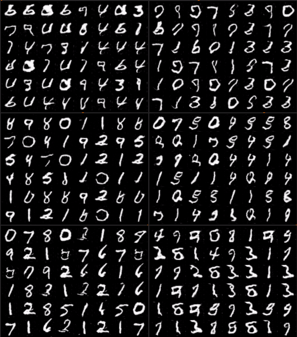
This one is looking much better than our previous model. In the next part, we will see another type of GAN called the W-GAN.