Generative Adversarial Networks Part 1 — An Introduction, and Implementation of the simplest form of GAN.
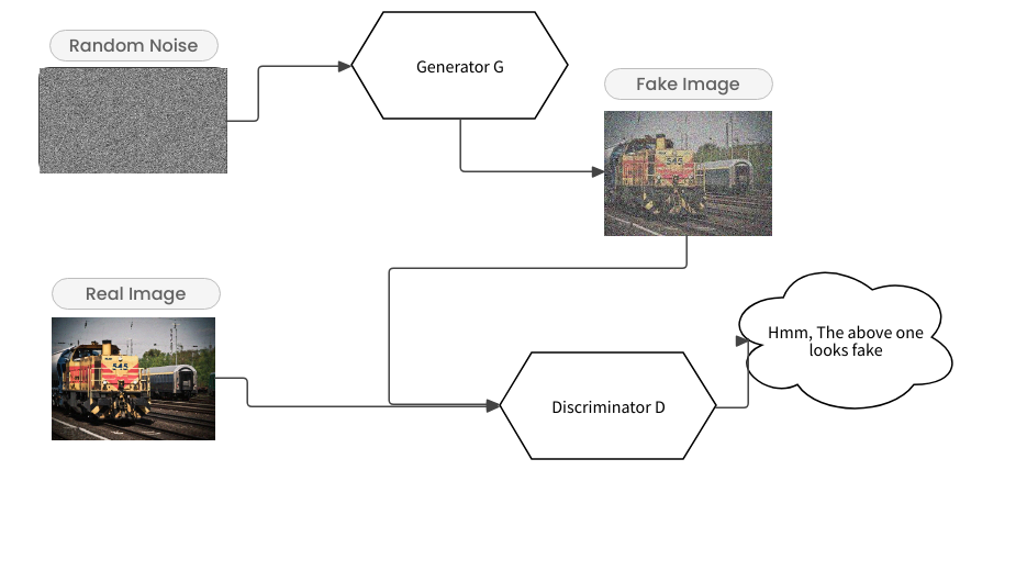
Generative Adversarial Networks, or GANs for short are generative modeling technique in deep learning which uses unsupervised learning algorithms to learn different patterns in the images.
The GANs typically consist of two models, one is the generator responsible for generating images from random noise, and the other is the discriminator, which keeps guessing whether the images generated by the generator are fake or real. The word Adversarial stands for this technique. This is like a min-max game between a generator and a discriminator where both of them try to dominate each other. The generator tries to fool the discriminator and the discriminator tries to keep guessing the fake images. The training continues at least until the generator becomes capable enough to fool the discriminator 50% of the time.
Let’s not go too deep into theoretical stuff since there are many internet resources explaining all this stuff so we will start implementing different kinds of these models.
In this part 1, we will implement and understand the simplest type of model, known as vanilla-GAN or S-GAN (Simple GAN). In this type of GAN, there is 1 generator and 1 discriminator and they play the game of adversarial as discussed above. Let’s take a look at the overall architecture first:
Now we will try to design the discriminator first since it is pretty straightforward, and then we will move on to designing the generator. Keep in mind no one implementation can be correct, there can be many different implementations for the same architecture. So now let’s hop onto our IDE and start designing.
Designing the Discriminator
The code that we are going to write in this article is also available on my GitHub repository The-Ultimate-GAN . If during this blog, something doesn’t work. You can open an issue on my GitHub repository and we can discuss the issue there.
We will be using PyTorch Library so let’s import the required libraries first.
import torch
from torch import nn
The nn stands for neural network and is a sub-module of the Pytorch library which provides different kinds of class implementations that may be required for building neural networks. Now that we have the libraries imported, let’s build a class for the Discriminator model. We will build a class and inherit it from the nn.Module from the Pytorch library. This is required since to create any layer, block, or module of any ML model, we need to inherit it from the nn.Module class. This gives it some predefined functions required for the neural network to work properly.
In this same block, we will create the __init__ function of the class and define our model architecture in it.
In this model, we are taking the img_dim as an init parameter. This parameter is the total number of pixels of the input image. In our case, since we are using mnist, our input size will be 28 x 28 x 1 = 784 input size or 784 img_dim.
Linear Layer
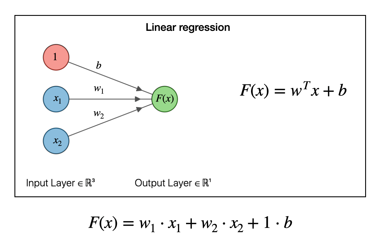
Now let’s deep dive into what this model architecture is and what each layer is exactly doing. First, we have a Linear layer. This corresponds to a very simple Linear layer with the linear function in which we do:
a = wX + b
Here we are providing it with two parameters. in_features and out_features . The in_features correspond to the total number of input pixels from the image. For example, let’s take the example of the mnist dataset. Each image in that dataset is 28 x 28 x 1 pixels. 28 x 28 is the height and width and 1 is the number of channels(The mnist dataset is in a grayscale format, not RGB format).
One sample image from the mnist dataset
Now what we do in the Linear layer is flatten out the image, which means we make each pixel of the image as an input feature called X. So the in_features corresponds to 28 x 28 x 1 = 784 input features. The out_features and the output from the Linear layer are 512 neurons.
Leaky ReLU
Then the second layer comes into play. The second layer is the LeakyReLU Layer. ReLU stands for Rectified Linear Unit. This layer is the activation layer which introduces a non-linearity in the neural network. The formula for Leaky ReLU is:
LReLU(x)=x if x⩾0 and (x×0.01) if x<0
Let’s see in detail what this formula means. We input the value of the neuron in this formula and according to its value we get the output e.g. if the value of two neurons is 2.1232 and -3.2123 respectively, then after passing through this layer the neurons will become 2.1232 since x > 0 and -0.032123 since x < 0 respectively. So you can see that we are left with positive values as they are and negative values are changed with a much smaller value thus providing a small gradient in the negative side also. To understand completely why we use the activation functions we will need a separate article. So let’s make that article a future goal.
Now that we understand the two fundamental layers, the next few layers are just a copy of these with some different parameters. You can notice that at every layer we are reducing the number of output features of the Linear Layer. This means that the information is being passed on and compressed into lesser and lesser features. Finally, at the last layer, you can see that we have in_features as 128 and out_features as 1. The 1 output feature corresponds to the image output as being fake or real so only 1 output. At the last layer of the discriminator, we have a sigmoid layer. Again this is an activation function with the property of scaling the input between 0 and 1. So the output stays between 0 and 1. 0 being fake and 1 being a real image.
You can visualize the model in your mind as – The first layer takes in input as pixel values, converts it into 512 features – Then a LeakyRelu adds nonlinearity – Then again a Linear layer that converts 512 into 256 features – Then a LeakyRelu adds nonlinearity to stabilize gradients – Then a Linear layer converts 256 into 128 features – Then Leaky Relu to add nonlinearity – Then Linear Layer which converts 128 into 1 output feature – Then a sigmoid function scales the output between 0 and 1.
This is it. This was our discriminator’s model. Now let’s create the function for inferencing this model i.e. passing the input from all these layers to get the output. We will overload the forward function, this function is inherited from the nn.Module class that we used earlier.
Nothing too fancy, we just pass the input x, which in this case will be the image flattened out, and pass it through the model. This will take the input and pass it through every layer to create an output i.e. the image is fake or real.
That’s it for the discriminator part. Pretty straightforward right? Now let’s move on to the generator which is somewhat difficult than the discriminator.
Designing the Generator
For the generator, we don’t need any extra library imports so let’s start writing the code for the generator.
Again, we first create a class inherited from the nn.Module class so it can be used as a neural network.
The Generator Block
We defined a function called the generator_block. The purpose of this function is to return us a single generator block which will be used as building blocks for creating a full generator. Let’s dive deep into the generator block.
First, we have the linear layer, the purpose of the linear layer and its working is already explained earlier so let’s move on ahead.
Batch Normalization
The second layer we have is the BatchNorm1d. This is the batch normalization layer and is a very important concept in Neural Networks. So let’s take a good look at it. First, let’s see the problem if we don’t use Batch Normalization. Consider we have a dataset of people of different ages and the number of miles they have driven. Now in the number of miles column, we will have some of the values as maybe 120 miles, or 130 miles, and some of the people may have driven 20000 miles or even 100000 miles. the difference in both values is huge. Similarly, there may be some people who are aged 25 and have driven thousands of miles and someone of 75 years of age and may have driven a few hundreds of miles. So the data is not consistent since the features with higher values like 100000 will get more attention in the neural network than smaller values. This makes it difficult for the neural network to learn and generalize patterns because the higher values will always get more attention. So for this purpose, we use something called Normalization. In simple normalization, we just take the mean and standard deviation of the dataset and this is the formula used:
Normalized(x) = (x — mean) / standard-deviation
This normalizes the input data, but what if after some deep layers, the features again become highly separated or in other words, the problem of internal covariate shift arises, this is where batch normalization comes in. Batch normalization introduces 4 new parameters for the neurons. Namely: 1. Running Mean (Non-trainable) 2. Running Covariance (Non-Trainable) 3. Gamma (γ) (Trainable) 4. Beta (β) (Trainable) The first two are simple mathematical calculations from the running data and apply the same normalization formula as discussed above. The main difference in batch norm is the two trainable parameters for each neuron. The Gamma γ is the scaling factor which determines how much to scale the layer and the Beta β is the shifting factor which tells how much to shift the layer. These parameters get trained during the Neural Network training process to find the optimal values for the γ and β.
Age vs Miles driven (Original vs Normalized)
We can see that in the normalized version, the values are close to each other with a standard deviation of one. This dataset tends to perform better since all the input features will get more attention. This is called Batch Normalization.
Getting back to the generator block, this layer helps normalize the data after the Linear layer. Now let’s move forward to the next layer.
Again, we have the LeakyReLU activation function which helps stabilize the gradients and improve generalization.
The complete Generator Block
Our generator function takes in 2 required parameters namely input_size and output_size and 1 additional parameter normalize which is by default set to True. Since we don’t need the normalization in the first layer because the data we pass on as input features are already normalized (We will see it later) the first block doesn’t need normalization so pass normalize as False. The input_size and output_size are again for the Linear layer and don’t require any additional explanation. We have a total of 4 generator blocks in our main generator model. After these generator blocks, we have two additional layers. One of them is the Linear layer which converts 1024 input features into an output image of size img_dim and in our mnist dataset case, it is 784.
After this, we have the TanH Activation function. This function is similar to the sigmoid function but outputs values between -1 and 1. The question here is why we need output between -1 and 1. This is because our input data is normalized using mean 0.5 and std 0.5. So our normalization function also outputs the data in range -1 and 1. We will see this further when creating the transforms for our data. This is it for our generator model. Now similar to the discriminator model, let’s make the forward function for our model:
Now let us start building the GAN with the generator and discriminator we built earlier. Let’s first import the libraries we need
import torch
import numpy as np
import torchvision
import os

from torch import nn
from torch import optim
from torchvision import datasets, transforms
from torch.utils.data import DataLoader
from torch.utils.tensorboard import SummaryWriter
from tqdm import tqdm
We will discuss these libraries on the go. First, let’s build a new class to wrap everything in:
This line sets device-agnostic code. If we have a GPU, the model will run on the GPU else if MPS is available, it will be used else the CPU will be used.
This is the transform function we talked about in the Tanh explanation. We can see here we are doing two things to each of the data point images. First, we convert it into a torch.Tensor object so it can be used in parallel computing code. Then we are applying normalization with mean and std as 0.5 and 0.5 respectively. So each input pixel will be converted in a range of -1 and 1 thus using the Tanh makes sense.
This is the fixed noise that will be used to evaluate the generator’s performance. Fixed noise so we can see how much better is the model performing compared to the last time.
Here we are doing a bunch of things, first, we are downloading the mnist dataset using the dataset from the torchvision library. torchvision provides different types of vision datasets to work with. We are setting the root directory so the dataset (if not available) will be downloaded to this folder. Then we set the original image shape to be used later. Our images are 28 x 28 and have 1 channel so we have (-1, 1, 28, 28) as the orig_shape. Lastly, we make a data loader with a given batch size for easy access to data. Dataloaders are a fundamental way to provide data to the ML models. More on that in some other article.
definit_generator(self, latent_dim, image_dim):
self.generator = Generator(latent_dim, image_dim).to(
self.device
) # Initialize the generatordefinit_discriminator(self, image_dim):
self.discriminator = Discriminator(image_dim).to(
self.device
) # Initialize the discriminatordefinit_optimizers(self, learning_rate):
self.opt_disc = optim.Adam(
self.discriminator.parameters(), lr=learning_rate
) # Initialize the discriminator optimizer
self.opt_gen = optim.Adam(
self.generator.parameters(), lr=learning_rate
) # Initialize the generator optimizerdefinit_loss_fn(self):
self.criterion = nn.BCELoss() # Initialize the loss functiondefinit_summary_writers(self):
self.writer_fake = SummaryWriter(
f"runs/GAN_{self.dataset_name}/fake"
) # Initialize the tensorboard writer for fake images
self.writer_real = SummaryWriter(
f"runs/GAN_{self.dataset_name}/real"
) # Initialize the tensorboard writer for real images
Nothing fancy, we are making objects of our discriminator, our Generator, initializing the optimizers (They update the parameters during training), and loss function. We are using the Binary Cross Entropy as the choice of our loss function. Let’s look deeper at why we are using the BCE Loss. The BCE Loss is given by
n = −w [ y ⋅ logx + (1 − y) ⋅ log(1 − x)]
and the Loss Function for the GANs, as mentioned by Ian Goodfellow in the 2014 research paper is a min-max function defined as :
Max (log( D(x) + log (1 — D(z)))
To achieve this, we are using the binary cross-entropy loss function. We will dig even deeper after we have written the training code so let’s move ahead for now. We are also initializing the summary writers. They are used to check the model scores in a presentable fashion using tensorboard which is a visualization library for the ML models. We will see it in action soon. Now let’s write the most important function, the train function.
deftrain(self):
try:
step = 0# Step for the tensorboard writerfor i inrange(self.num_epochs): # Loop over the dataset multiple timesfor batch_idx, (real, _) inenumerate(tqdm(self.loader)):
real = real.view(-1, np.prod(self.image_shape)).to(self.device)
batch_size = real.shape[0]

noise = torch.randn(batch_size, self.latent_dim).to(self.device)
fake = self.generator(noise)  # Generate fake images
discriminator_real = self.discriminator(real).view(-1)
lossD_real = self.criterion(discriminator_real, torch.ones_like(discriminator_real))
discriminator_fake = self.discriminator(fake).view(-1)
lossD_fake = self.criterion(discriminator_fake, torch.zeros_like(discriminator_fake))
lossD = (lossD_real + lossD_fake) / 2# Calculate the average loss for the discriminator
self.discriminator.zero_grad() # Zero the gradients
lossD.backward(retain_graph=True) # Backward pass for the discriminator
self.opt_disc.step() # Update the discriminator weights
output = self.discriminator(fake).view(-1)  # Get the discriminator output for fake images
lossG = self.criterion(output, torch.ones_like(output))  # Calculate the loss for the generator
self.generator.zero_grad()  # Zero the gradients
lossG.backward()  # Backward pass for the generator
self.opt_gen.step() # Update the generator weightsif batch_idx == 0:
print(f"Epoch [{self.current_epoch}/{self.num_epochs}] Loss Discriminator: {lossD:.8f}, Loss Generator: {lossG:.8f}")
with torch.no_grad(): # Save the generated images to tensorboard
fake = self.generator(self.fixed_noise).reshape(
self.orig_shape
) # Generate fake images
data = real.reshape(self.orig_shape) # Get the real images
img_grid_fake = torchvision.utils.make_grid(
fake, normalize=True
) # Create a grid of fake images
img_grid_real = torchvision.utils.make_grid(
data, normalize=True
) # Create a grid of real images
self.writer_fake.add_image(
f"{self.dataset_name} Fake Images",
img_grid_fake,
global_step=step,
) # Add the fake images to tensorboard
self.writer_real.add_image(
f"{self.dataset_name} Real Images",
img_grid_real,
global_step=step,
) # Add the real images to tensorboard
step += 1# Increment the step
Okay, let’s look at individual lines of code now. We are iterating through each epoch and in each epoch, we are iterating through each batch of the data using the self.loader we made earlier. It divides the data into smaller chunks of batch_size.
Here, we are just flattening out the real image into a one-dimensional array of size 784 (since img_size is (28, 28, 1). Then we get the batch size although we can use the one we defined earlier. After that, we create a random noise of size latent_dim. This noise then passes through each layer of the generator to give a final image. The size we set for latent_dim or in other words the noise size is 64. So it will create a tensor of size (32, 64) where 32 is the batch_size. Finally, we pass this noise through the generator to get a fake image.
Training the Discriminator
discriminator_real = self.discriminator(real).view(-1)
lossD_real = self.criterion(discriminator_real, torch.ones_like(discriminator_real))
discriminator_fake = self.discriminator(fake).view(-1)
lossD_fake = self.criterion(discriminator_fake, torch.zeros_like(discriminator_fake))
lossD = (lossD_real + lossD_fake) / 2# Calculate the average loss for the discriminator
self.discriminator.zero_grad() # Zero the gradients
lossD.backward(retain_graph=True) # Backward pass for the discriminator
self.opt_disc.step() # Update the discriminator weights
Here we are giving the discriminator, real image, and fake image in lines 1 and 3 respectively. The discriminator outputs what it thinks of both the images, then we use them in the BCE Loss. This is a bit tricky. We saw earlier that we are trying to maximize:
Max (log( D(x) + log (1 — D(G(z))))
Now to find log(D(x)) we use the BCE Loss. In the BCE loss,
n = −[ y ⋅ logx + (1 − y) ⋅ log(1 − x)]
we are passing x as the D(real) or discriminator_real and passing y as torch.ones_like(discriminator_real). What this means is when y will be 1, we put it in the above BCE Loss equation and are left with log x. Since (1 — y) will become zero and cancel the second term out. Similarly, to find log(1-D(G(z))) we pass the discriminator_fake
as x and torch.zeros_like(discriminator_fake)) as y. With this, we are left with log(1 — x) since y will be zero and cancel the other term out. So we are left with the above equation we are trying to maximize. Finally, we call the zero_grad function on the discriminator and step the optimizer to update the weights.
Training the Generator
output = self.discriminator(fake).view(-1) # Get the discriminator output for fake images
lossG = self.criterion(output, torch.ones_like(output)) # Calculate the loss for the generator
self.generator.zero_grad() # Zero the gradients
lossG.backward() # Backward pass for the generator
self.opt_gen.step() # Update the generator weights
For the generator, we are doing something similar. We are trying to
maximize log(D(G(z)))
So we pass in the output from the generator as x and y as 1 again and we are left with log (D(G(z))) (You can input y in the BCE Loss to verify). Then again, calling zero_grad on the generator and stepping the optimizer to update the generator weights.
Outputs for the tensorboard
We are almost done with all the technical stuff, the following code is to output the losses and create image grid for the tensorboard
if batch_idx == 0:
print(f"Epoch [{self.current_epoch}/{self.num_epochs}] Loss Discriminator: {lossD:.8f}, Loss Generator: {lossG:.8f}")
with torch.no_grad(): # Save the generated images to tensorboard
fake = self.generator(self.fixed_noise).reshape(
self.orig_shape
) # Generate fake images
data = real.reshape(self.orig_shape) # Get the real images
img_grid_fake = torchvision.utils.make_grid(
fake, normalize=True
) # Create a grid of fake images
img_grid_real = torchvision.utils.make_grid(
data, normalize=True
) # Create a grid of real images
self.writer_fake.add_image(
f"{self.dataset_name} Fake Images",
img_grid_fake,
global_step=step,
) # Add the fake images to tensorboard
self.writer_real.add_image(
f"{self.dataset_name} Real Images",
img_grid_real,
global_step=step,
) # Add the real images to tensorboard
step += 1# Increment the step
Nothing fancy, just creating some fake images from the fixed noise we defined earlier. The reason was so generator, while evaluating, always gets the same noise so we know how much it has improved. Then we make the grids and write this grid data into the respective folders created in the runs folder. We will see it in action soon.
Wooh! That was a lot of code and theory, now let’s see our model in action. We will make the model object, pass in some parameters, and call its train function to see it in action.
model = SimpleGAN(
        learning_rate=3e-4,
        latent_dim=64,
        batch_size=32,
        num_epochs=50,
    )
model.train()
This will first download the dataset MNIST and then start training the model. If you see some library import errors like:
No library named tensorboard
or something like that, just run the following command on the command line
Here you will see the updated images every epoch. If for some reason the images don’t update, you can check your settings by going to the upper right corner and changing the setting of auto-reload. We can see that our model improves with time:
GIF showing model improvement over several epochs
This is it for this blog, enjoy your first GAN model. In the next part, we will see another type of GAN called the DC-GAN.